• Programming
• Physics
• Design
• Interactivity
• Function List

Programming Modelian

Basic Programming

Defining Variables

Modelian allows the definition and modification of variables using the "<-" operator. For instance, the following code will create two variables — x and xSquared — which will be 20 and 100 respectively at the end of the code's evaluation.

x <- 10
xSquared <- x^2
x <- x*2

Modelian uses block scoping so variables first declared within a block will not be accessible outside that block.

Comments

Modelian supports several forms of comments. Comments are parts of equations that will not be evaluated by the equation engine:

• "#" will comment out the rest of the line:

  1+2^3 # this is ignored

• "//" will comment out the rest of the line:

  1+2^3 // this is ignored

• "/*" and "*/" will comment out a region:

  1+/* this is ignored */2^3

Defining Functions

Modelian supports several forms for function definition. One is a short form that is shown below:

myFn(a, b, c) <- sin((a+b+c)/(a*b*c))

And the second is a longer form that can create multi-line functions:

function myFn(a, b, c) 
   numerator <- a+b+c 
   denominator <- a*b*c 
   sin(numerator/denominator) # the last evaluated expression is returned from a function, you may also use the 'return' statement
end function

Functions also support default parameter values:

takePower(a, b = 2) <- a^b

takePower(2, 1) # = 2
takePower(3, 3) # = 27
takePower(3) # = 9

If Then Else Statements

In addition to Modelian's standard ifThenElse() function, a multi-line form is also supported:

if x > 10 then
   # do something
else if x < 5 then
   # do something else 
else
   # some other action
end if 

You may have as many "else-if"clauses as desired and the final "else" clause is optional.

While Loops

While loops allow the repetition of expressions multiple times until as long as a logical condition is satisfied. For example:

x <- 10
while x < 20
   x <- x +x/10
end loop
x # = 21.436

For Loops

For loops repeat some code a fixed number of times. For instance:

total <- 0 
for x from 1 to 10 
   total <- total + x 
end loop
total # = the sum of the numbers from 1 to 10

An optional "by" control parameter can be specified to change the step to some other value than one:

total <- 0 
for x from 1 to 9 by 2
   total <- total + x
end loop
total # = the sum of the odd numbers from 1 to 9

A special form of the for loop, the for-in loop, exists for iterating across all elements of a vector:

total <- 0 
for x in {1, 2, -5, 10}
   total <- total + x
end loop 
total # sums up the elements in the vector

Returning Values

A return statement may be used to return values from functions or equations. If a return statement is not used, the last evaluated expression will automatically be returned.

For example:

1+1
2+2
3+3 # 6 will be returned by this equation

Or:

1+1
return 2+2 # 4 will be returned by this equation
3+3 # this won't be evaluated

Or:

if 10 > 20 then
   1*2
else
   2*2 # 4 is returned from both the if-statement and then returned for the expression overall
end if

Destructuring Assignment

Modelian supports destructuring assignment. Though the name is fancy, the concept is simple. Basically, destructuring assignment provides a straightforward way to assign the elements of a vector to a set of variables. For example:

x, y <- {10, 20}
x # = 10
y # = 20

Functional Programming

Functional programming is a approach to programming that focuses on the use of functions rather than variables and procedural logic. Modelian supports functional programming as its functions are first class objects that can be created on the fly, assigned to variables, and returned as the results of other functions.

For instance, we could take the built in Mean() function, assign it to a variable and then apply it to a set of numbers:

Similarly, we could use the Map function with a vector of functions to calculate summary statistics for a set of data values:

{Min, Median, Max}.Map(x(7, 5, 8, 1, 6)) # = {1, 6, 8}

Anonymous Functions

Generally, when programming a function is given a name when it is created and it can later be referred to using that name. In functional programming, a key tool are anonymous functions: functions created without a name. Anonymous functions are defined much the same way as regular functions, but without an explicit name. For instance, the following creates an anonymous function and assigns it to the variable f:

f <- function(x,y)
   Sqrt(x^2+y^2)
end function

f(3, 4) # = 5

There is also a shorthand syntax available for single line anonymous functions:

f <- function(x,y) Sqrt(x^2+y^2)

f(3, 4) # = 5

Anonymous functions are very useful when using functions like Map() and Filter(). For instance:

{1, 2, 3}.map(function(value)
   cos(value^2)
end function)

Closure

Closure is a key tool for functional programming. Closure is a bit of a technical concept which basically means that functions declared within a scope continue to have access that scope even after it has been released. Let us look at an example that uses closure to generate counter functions:

function MakeCounter()
   countTally <- 0
   function()
      countTally <- countTally+1
      countTally
   end function
end function

c1 <- MakeCounter()
c2 <- MakeCounter()

{c1(), c1(), c2(), c2(), c1()} # = {1, 2, 1, 2, 3}

Looking at this code we should recognize that countTally is a local variable to the MakeCounter function. Once the function is complete, the countTally variable goes out of scope and we cannot access it outside the function. However, due to closure, the function we declare within the MakeCounter function still has access to the countTally variable even after MakeCounter has finished

Thus we can continue to use the countTally variable in this anonymous function when we call it later on. It is effect now a private variable that only the generated function can access. A new countTally variable is created for each call of MakeCounter, so we can keep track of separate counts. Closure is a powerful tool that has many uses for complex programs

The Elegance of Functional Programming

Functional programming techniques are really quite elegant for many practical programming uses. Take the following example which implements the Lotka-Volterra predator prey model using Modelians programming features. Euler's method is used to solve the differential equations. Due to the elegance of functional programming, once we have defined our system, the entire differential equation solver requires just a single loop containing only two lines of code!

state <- {
    Predator: 20,
    Prey: 560
}

derivatives <- {
    Predator: function(state) 0.0002*state.Prey*state.Predator-0.25*state.Predator,
    Prey: function(state) 0.25*state.Prey-0.008*state.Predator*state.Prey
}

startTime <- 0
endTime <- 20
timeStep <- 1

for t in startTime:timeStep:(endTime-timeStep)
    slopes <- derivatives.map(x(state))
    state <- state + slopes*timeStep
end loop

alert(state)

Object Oriented Programming

Object oriented programming is a technique where objects are defined in a program. These objects are generally collections of properties and functions that may manipulate the object or carry out some behavior based on the object's state. Modelian's equation engine supports what is known as prototype-based object oriented programming. This is a flexible and powerful technique for building programs using objects.

Creating Objects

Object are based on vectors. Let's take the following instance as an example:

Person <- {
   firstName: "John",
   lastName: "Smith"
}

This object, represents a person named John Smith. We can access this person's first and last name using the following syntax:

Person.firstName # = "John"
Person.lastName # = "Smith"

Since Modelian's equation engine is a functional language with first class functions, we can also assign functions to the properties of this object. For instance, we could add a function to return the person's full name:

Person <- {
   firstName: "John",
   lastName: "Smith",
   fullName: function()
      "John Smith"
   end function
}

We would then obtain the full name of the person object like so:

Person.fullName() # = "John Smith"

However, this function we wrote is not very smart. Our object already has all the information needed to find the person's full name, so repeating the name in the function is redundant. We can do better than this. To do so, we use a special variable: Self. When used in an object's function, Self refers to the object itself. Using this knowledge, we can rewrite our full name function to be smarter. In this new form, the full name function will give the correct full name even if we later change the object's first or last name.

Person <- {
   firstName: "John",
   lastName: "Smith",
   fullName: function()
      self.firstName+" "+self.lastName
   end function
}

Inheritance

Unlike some language, in Modelian each object is both a fully usable object and also a class definition other objects can inherit from. We use the new keyword to create instances of existing objects.

For example, we could create two new people objects like so:

chris <- new Person
chris.fistName <- "Chris"
john <- new Person

chris.firstName # = "Chris"
john.firstName # = "John"

You can also create multiple levels of inheritance. For instance, imagine we wanted to create a Student class. The Student class will be a subclass of the person class with two new properties: school and grade.

Student <- new Person
Student.grade <- 10
Student.school <- "Midfield High"

chris <- new Student # Chris is both a Student and a Person

Constructors

Constructors are functions that are called when a new instance of a class is created. Constructors are created by defining a property "constructor" in the object definition. If a constructor is available it will be called when the a new instance of an object is created. For instance, the following is a constructor that makes it easy to create people with a given name:

Person <- {
   firstName: "John",
   lastName: "Smith",
   fullName: function() self.firstName+" "+self.lastName,
   constructor: function(first, last)
      self.firstName <- first
      self.lastName <- last
   end function
}

chris <- new Person("Chris", "McDonald")
chris.fullName() # = "Chris McDonald"

Monkey-Patching

All classes in Modelian are fully dynamic. This means that you can add properties to the class definition and all instances (current and future) of that class will immediately have access to those properties. This is sometimes known as "Monkey Patching". This capability extends to Modelian's internal classes. For instance, all strings in Modelian inherit from the StringBase object and all vectors inherit from the VectorBase object. We can modify these objects to extend Modelian functionality.

As an example, let's extend Modelian strings with a Reverse() function. Such a function is not built into Modelian but it might be nice to have. Let's give it a try:

StringBase.reverse <- function()
   self.range(self.length():1)
end function

"Test".reverse() # = "tseT"

Parent

The object an instance inherits from is known as its Parent. A variable by this name is available in the object's functions in order to obtain a reference to the object's parent. This is especially useful for stringing constructors together. For instance, we may want to create a Student subclass of Person which calls its parent constructor:

Student <- new Person("","")
Student.grade <- 10
Student.school <- "Midfield High"
Student.constructor <- function(first, last, grade, school)
   self.grade <- grade
   self.school <- school
   parent.constructor(first, last)
end function

Physics

Modelian is based on a rigid-body physics simulation. This simulation is powered by the Box2D simulation engine. Modelian simulates the interactions between various objects in a physically realistic environment. The Modelian world is defined in cartesian coordinates with units of meters, kilograms and seconds where (0, 0) is the bottom center of the screen. The screen spans from -5 meters to 5 meters in width and the y-position increases as you move upwards.

Modelian supports the following physical properties of objects:

• Size and Geometry
• Linear and Angular Velocity
• Density
• Springiness (restitution)
• Friction

You can create objects using the Create function and then configure their geometries or properties:

obj <- create() # Creates an object
obj.setSides(2, 1) # Sets the geometry of the object to a rectangle with a width of 2 meters and a height of 1 meter
obj.setDensity(10) # Makes the object dense

Most of Modelian functions can operate on vectors of objects in addition to a single object. So the following function will create 5 boxes and change all their densities:

obj <- repeat(create(), 5) # Creates a vector of five objects 
obj.setDensity(10) # Makes all the objects dense

Modelian has built-in support for units and automatic unit conversions. Units are denoted using two angle brackets: '{' '}'. The following are examples of usages of units.

{1 Meter}/{10 Seconds} # = 0.1 Meters per Seconds
{2 Meters}+{5 Centimeters} # = 2.05 Meters
{2 Meters}+{5 Seconds} # Error: Invalid unit conversion

Modelian's built-in functions accept and return numbers with units. If you pass a unitless number to one of Modelian's built-in functions, it will be converted to the Meters-Kilograms-Seconds unit system.

See all physics functions

Design

You may style objects by changing their colors and optionally assigning an image for an object.

Colors may be set using the SetColor and SetLineColor functions which will set the fill and line colors of an object respectively. Colors may be specified either using a vector of fractional red, green, blue components; or using a color name. For example the following creates a red object with a green outline. The SetBackgroundColor function may be used to set the background of the program.

p <- create()
p.setColor("red")
p.setLineColor(p, {0, 1, 0})

The following is a list of available color names:

"black"
"navy"
"darkblue"
"mediumblue"
"blue"
"darkgreen"
"green"
"teal"
"darkcyan"
"deepskyblue"
"darkturquoise"
"mediumspringgreen"
"lime"
"springgreen"
"aqua"
"cyan"
"midnightblue"
"dodgerblue"
"lightseagreen"
"forestgreen"
"seagreen"
"darkslategray"
"darkslategrey"
"limegreen"
"mediumseagreen"
"turquoise"
"royalblue"
"steelblue"
"darkslateblue"
"mediumturquoise"
"indigo "
"darkolivegreen"
"cadetblue"
"cornflowerblue"
"mediumaquamarine"
"dimgray"
"dimgrey"
"slateblue"
"olivedrab"
"slategray"
"slategrey"
"lightslategray"
"lightslategrey"
"mediumslateblue"
"lawngreen"
"chartreuse"
"aquamarine"
"maroon"
"purple"
"olive"
"gray"
"grey"
"skyblue"
"lightskyblue"
"blueviolet"
"darkred"
"darkmagenta"
"saddlebrown"
"darkseagreen"
"lightgreen"
"mediumpurple"
"darkviolet"
"palegreen"
"darkorchid"
"yellowgreen"
"sienna"
"brown"
"darkgray"
"darkgrey"
"lightblue"
"greenyellow"
"paleturquoise"
"lightsteelblue"
"powderblue"
"firebrick"
"darkgoldenrod"
"mediumorchid"
"rosybrown"
"darkkhaki"
"silver"
"mediumvioletred"
"indianred "
"peru"
"chocolate"
"tan"
"lightgray"
"lightgrey"
"thistle"
"orchid"
"goldenrod"
"palevioletred"
"crimson"
"gainsboro"
"plum"
"burlywood"
"lightcyan"
"lavender"
"darksalmon"
"violet"
"palegoldenrod"
"lightcoral"
"khaki"
"aliceblue"
"honeydew"
"azure"
"sandybrown"
"wheat"
"beige"
"whitesmoke"
"mintcream"
"ghostwhite"
"salmon"
"antiquewhite"
"linen"
"lightgoldenrodyellow"
"oldlace"
"red"
"fuchsia"
"magenta"
"deeppink"
"orangered"
"tomato"
"hotpink"
"coral"
"darkorange"
"lightsalmon"
"orange"
"lightpink"
"pink"
"gold"
"peachpuff"
"navajowhite"
"moccasin"
"bisque"
"mistyrose"
"blanchedalmond"
"papayawhip"
"lavenderblush"
"seashell"
"cornsilk"
"lemonchiffon"
"floralwhite"
"snow"
"yellow"
"lightyellow"
"ivory"
"white"

Images may be specified for objects. The SetBackgroundImage function may be used to set the background for the program. The following are available background images:

Background Images

"autumn"
"beach"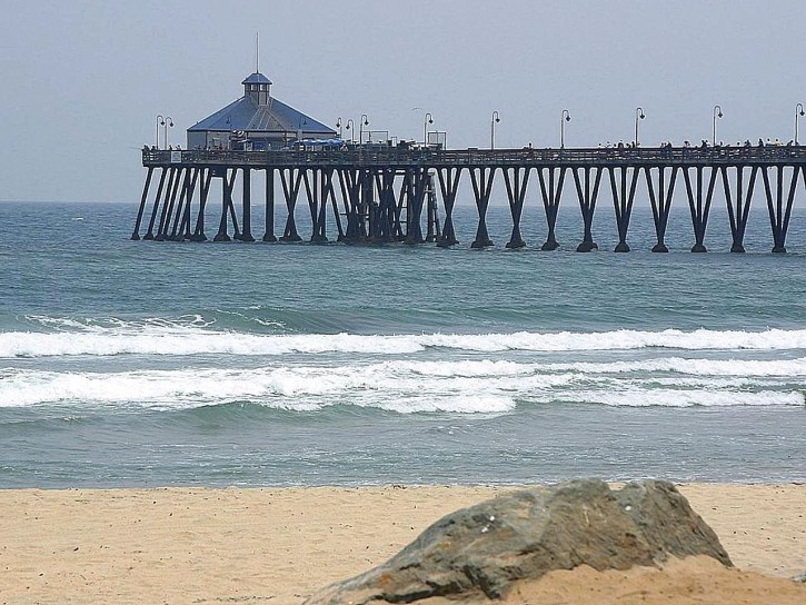
"bridge"
"christmas"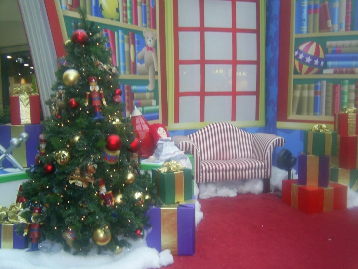
"clouds"
"field"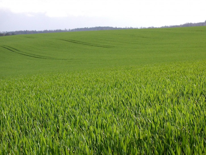
"fireworks"
"forest"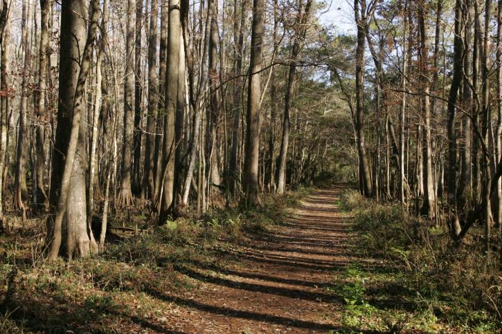
"galaxy"
"island"
"lasvegas"
"mist"
"moon"
"mountain"
"seacave"
"singapore"
"snow"
"stars"
"underwater"
"volcano"
"waterfall"

The SetImage function can be used to set the image for an object. Any image can be used on any object. However, if the geometry of the object does not match the image, collisions and physics might not match what is displayed. The following are available object images:

Object Images

"asteroid"
"basketball"
"beachball"
"blackglass"
"blueblock"
"brick"
"crate"
"diamond"
"discoball"
"earth"
"eightball"
"golfball"
"greenblock"
"greyglass"
"grin"
"heart"
"home"
"kiss"
"mars"
"poweroutlet"
"redblock"
"saucer"
"smile"
"smiley"
"soccerball"
"sunglasses"
"tennisball"
"toxic"
"warning"
"wheel"
"wink"

See all design functions

Interactivity

Modelian supports mouse and keyboard interactivity using an event callback model. In short, you specify a function to carry out an action when an event occurs. Then you register that function as an event handler using, for instance, the OnKeyDown function. The following is an example of interactivity that creates a new object every time the user clicks their mouse.

Function CreateObject(event)
   obj <- create()
   obj.setPosition(event.x, event.y)
End Function
OnMouseDown(CreateObject)

Many types of events can also be assigned directly to objects. These events are different from global events in that they will only be executed when the user is interacting with the object. For instance, the following code will create an object and set its color to red when the user clicks on it. If the user clicks anywhere else than the object itself, their click will have no effect on the object

ball <- create()
ball.onClick <- function() self.setColor("red")

Keyboard related functions use keycodes to report which key is pressed. This table may be used to look up the keycode for different keys.

See all interactivity functions

List of Functions